
Types of statistical distributions in ml will be described in this article. Statistical distributions are highly helpful in data science and machine learning because they provide a range of possible values for the variables, which helps us understand an issue better. These seven distribution types, which frequently appear in real-world data, are illustrated with clear examples.
Probability and distributions are used in many facets of life to assess the likelihood of events, whether you’re speculating about whether it will rain tomorrow, wagering on a sports team to win an away game, drafting an insurance policy, or just trying your luck at blackjack.
Top 7 Types Of Statistical Distributions With Practical Examples
In this article, you can know about Types of statistical distributions here are the details below;
A data scientist’s daily work might greatly benefit from having a strong background in statistics. One of the fundamental components of machine learning and data science is probability. Although probability allows us to perform mathematical computations, statistical distributions enable us to see the underlying dynamics.
Finding patterns in a new dataset and analyzing it become much simpler when one has a solid understanding of statistical distribution. It expedites the procedure overall and aids in selecting the best machine learning model to suit our data on.
PRO TIP: To improve your data science skill set, enroll in our data science bootcamp program right away!
We will discuss common distributions for various data types in this blog, along with fascinating real-world application examples.
Common types of data
Gaining knowledge about the kind of data that different distributions employ makes explaining them easier. In our daily experiments, we come across two distinct outcomes: finite and infinite outcomes.

There are only so many ways a die can roll or a card can be chosen from a deck. Discrete data is a sort of data that has a limited set of possible values. For instance, the values that must be entered when rolling a die are 1, 2, 3, 4, 5, and 6. Also check Is This Website Safe complete guide
In a similar vein, our everyday surroundings provide instances of endless results from discrete occurrences. There are countless values that can be recorded in a given interval whether measuring someone’s height or recording time. Continuous data is a type of data that can have any value within a specified range. Both finite and limitless ranges are possible.
Let’s say you weigh a watermelon, for instance. Any figure between 10.2 kg and 10.24 kg or 10.243 kg is possible. Making it continuous since it is measurable but not countable. Conversely, let’s say you count the number of boys in a class; this value is discrete because it is countable.
Types of statistical DISTRIBUTIONs
We have classified distributions into two categories: discrete distributions for discrete data (limited outcomes) and continuous distributions for continuous data (infinite outcomes), depending on the type of data we utilize.
Discrete distributions
Discrete uniform distribution:
Every possible result has the same probability
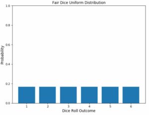
A uniform distribution is a statistical distribution that has an equal probability of every possible result. Think about throwing a six-sided die. On your subsequent roll, you have an equal chance of getting all six numbers, that is, a probability of 1/6 if you get exactly one of the following: 1, 2, 3, 4, 5, or 6. This is an example of a discrete uniform distribution.
Consequently, every possible outcome is represented by equal-height bars on the uniform distribution graph. The height in this scenario has a chance of 1/6 (0.166667).
The function U(a, b), where a & the b stand for the beginning and ending values, respectively, represents a uniform distribution. For continuous variables, there is a continuous uniform distribution that is comparable to a discrete uniform distribution.
This distribution’s shortcomings include the fact that it frequently gives us no pertinent information at all. Since there is no such thing as half a number on a dice, using our example of a rolling die, we obtain the predicted value of 3.5, which provides us with no accurate intuition. It doesn’t really help us predict anything because every value has the same likelihood.
One of the simplest distributions to comprehend is the Bernoulli distribution. It can serve as a foundation for obtaining more intricate distributions. A Bernoulli distribution applies to any event with a single trial and only two possible outcomes. Examples of a Bernoulli distribution are flipping a coin or selecting True or False in a test.
There is just one trial and two possible results. Assuming a single coin flip, there will be just one trail. Either heads or tails are the only two possible results. An illustration of a Bernoulli distribution is this one.
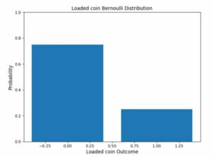
When employing a Bernoulli distribution, we typically have the likelihood of one of the possible outcomes (p). By subtracting (p) from the total probability (1), which is represented as (1-p), we can get the likelihood of the opposite outcome.
The likelihood of success, denoted by p, is given by the expression bern(p). E(x) = p represents the expected value of a Bernoulli trial, while Var(x) = p(1-p) represents the Bernoulli variance.
Bernoulli distribution
A Bernoulli distribution’s graph is easy to read. There are just two bars in it; one grows to the corresponding probability p, and the other to 1-p.
Distribution Binomial: A series of Bernoulli phenomena
The total results of an event that follows a Bernoulli distribution can be compared to the Binomial Distribution. As a result, in binary outcome events, the Binomial Distribution is employed, and the likelihood of success or failure remains constant over all subsequent trials. To count the number of heads and tails after flipping a coin several times is an example of a binomial event.
Bernoulli versus binomial distribution.
An example explains how these distributions differ from one another. Imagine you are taking a quiz with ten True/False questions. A single T/F question attempted would be referred to as a Bernoulli trial, whereas trying all ten of the T/F questions on the quiz would be called a Binomial trial. The following are the primary traits of the binomial distribution:
Each trial is independent of the others when there are several of them. In other words, one trial’s result has no bearing on subsequent ones.
There are simply two possible outcomes (winning or losing), with probabilities p and (1 – p), for each trial.
B (n, p), where n is the digit of trials and p represents the chance of success in a single trial, is the representation of a binomial distribution. Since a Bernoulli distribution has a single trial, it can be formed as a binomial trial with the formula B (1, p). E(x) = np, or the number of times a success occurs, is the expected value of a binomial trial “x”. Likewise, Var(x) = np(1-p) is used to express variance.
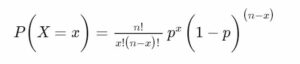
Let’s look at the number of trials (n) and the likelihood of success (p). Then, we can use the following formula to get the chance of success (x) for these n trials:
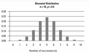
Binomial distribution
Assume, for illustration purposes, that a confectionery company makes candy bars with both milk and dark chocolate. There are half milk chocolate bars and half dark chocolate bars in the entire offering. Let’s say you pick ten candy bars at random, and selecting milk chocolate is what’s considered successful. The binomial distribution graph below displays the probability distribution of the number of sensations during these ten trials with p = 0.5:
Poisson Distribution:
The Poisson distribution describes how frequently an event happens during a given interval. With Poisson distribution, the frequency of an event over a certain time or distance is required, not its probability. A cricket, for instance, chirps twice every seven seconds on average. We can calculate the possibility that it will chirp five times in 15 seconds using the Poisson distribution.
The formula Po(λ), where λ is the predicted number of events that can occur in a period, is used to describe a Poisson process. A Poisson process’s variance and expected value are both equal to λ. The discrete random variable is denoted by X. This formula can be used to simulate a Poisson Distribution.
The following are the primary traits that characterize Poisson Processes:
- The happenings don’t depend on one another.
- Any number of occurrences (within the specified period) can occur for an event.
- No two things can happen at the same time.
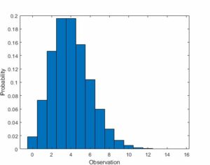
The Poisson distribution graph shows the probability of each occurrence as well as the number of times it occurs within a given time frame.
Constant distributions
In data science, the normal distribution is the most commonly used distribution. Data in a network with a normal distribution is symmetrically distributed and skew-free. Plotting the data reveals a bell-shaped distribution, with the majority of values centered around the center and dropping off as values move outward.
In nature and life, the normal distribution is commonly found in a variety of forms. An exam’s scores, for instance, have a normal distribution. As seen in the graph below, several of the pupils received scores in the range of 60 to 80. Students who score outside of this range are obviously not in the middle.
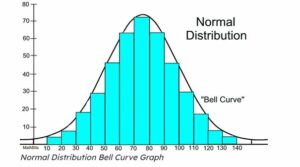
This shows the “bell-shaped” curve encircling the central area, which denotes the location of the majority of data points. Here, the normal distribution is denoted by the notation N(µ, σ2), where σ2 is the variance and µ is the mean, one of which is mostly supplied. A normal distribution’s mean equals its anticipated value. Several attributes can aid in identifying a normal distribution, including:
At the center, the curve exhibits symmetry. As a result, all values are distributed symmetrically about the mean, with the mean, mode, and median all equal to the same value.
Since all of the probabilities must add up to 1, the area under the distribution curve equals 1.
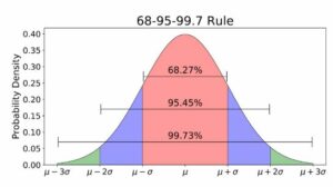
Rule 68-95-99.7
68% of all values on a graph representing a normal allocation fall within one standard deviation of the mean. In the aforementioned example, 68% of the values fall between 60 and 80 if the mean is 70 and the standard variation is 10. Comparably, 99.7% of the values are within three standard deviations of the mean, and 95% of the values are within two standard deviations. Almost everything is captured in this final moment. A data point is most likely an outlier if it is not included.
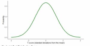
graph Probability Density and Student t-Test Distribution according to the 68-95-99.7 Rule: Approximation of a normal distribution with a small sample size
The student’s t-distribution, sometimes referred to as the t distribution, is a kind of statistical distribution that resembles the normal distribution in that it has heavier tails but a bell-shaped form. When sample sizes are tiny, the t distribution is utilized rather than the normal distribution.
Student t-Test Distribution
Let’s take an example where we are dealing with a shopkeeper’s monthly total of apples sold. The normal distribution will be applied in the scenario. On the other hand, the t distribution can be used if we are working with a smaller sample, such as the total number of apples sold in a day.
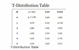
The requirement to define the distribution’s degrees of freedom in addition to the mean and variance is another significant distinction between the students’ t distribution and the normal one. The number of values that can vary in a statistic’s final calculation is known as its degree of freedom in statistics. T(k), where k is the number of degrees of freedom, is the representation of a student’s t distribution. When there are two degrees of freedom, or k=2, the expected value and the mean are equal.
All things considered, the student t distribution is commonly employed in statistical analysis and is crucial for carrying out hypothesis testing with sparse data.
One of the most popular continuous distributions is the exponential distribution. It is employed to simulate the intervals of time between various events. For instance, it is frequently used to quantify radioactive decay in physics, the time it takes to receive a defective item on an assembly line in engineering, and the probability of the next default for a portfolio of financial investments in finance. Exponential distributions are also frequently used in survival analysis (e.g., estimated life of a machine/device).
To learn about statistics, pick up one of the top ten statistics books.
Exp(λ), where λ is the distribution parameter—also referred to as the rate parameter—is a typical way to express the exponential distribution. The formula = 1/μ, where μ is the mean, can be used to determine the value of λ. In this case, the mean and standard deviation are the same. The variance is granted by Var (x) = 1/λ2.
exponential distribution curve on a graph
A curved line that depicts the exponential change in probability is called an exponential graph. When calculating a product’s lifetime or reliability, exponential distributions are frequently employed.
Conclusion
The process of developing models and doing data exploration requires data. Examining the data distribution is the first thing that comes to mind when working with continuous variables. If we can find the pattern in the data distribution, we may modify our Machine Learning models to better fit the situation, which shortens the time it takes to produce an accurate result.
In fact, certain machine learning models are designed to function optimally under specific distribution assumptions. So, knowing which distributions we’re working with could help us choose the right models to use.